 Geoactive
Latest Release: IC 2024 now available!
The latest version of Interactive Correlations (IC), our multi-well collaboration software, is now available. With two decades of continuous software...

The North Sea has a wealth of history in the exploration and production of oil and gas. It can be easy to assume that, with the number of wells, history and data from the region, there is nothing left to find, or nothing new to learn. As an Explorationist, would you agree?
Harbour Energy is playing a role in meeting the world's energy needs through sane, efficient and responsible production of hydrocarbons. They are focused on maintaining a portfolio of reserves and resources. This case study is focused on the investigation into the remaining potential within the Paleocene Play of the Norwegian Central Graben in the North Sea.
Directly Download this Case Study
Building upon the Facies Map Browser (FMB) data from TGS with additional data from multiple sources from across the UK and Norway wells in the Central Graben resulted in the understanding of some areas with potential that require further investigation. Specifically, the FMB data was used for quick overviews of regional distribution of the Paleocene zones. This allowed assignment of chance of success for the Paleocene across the area. Integrating the Reservoir, Seal and Source story from these wells can highlight the areas with a potentially higher chance of success as previously mapped.
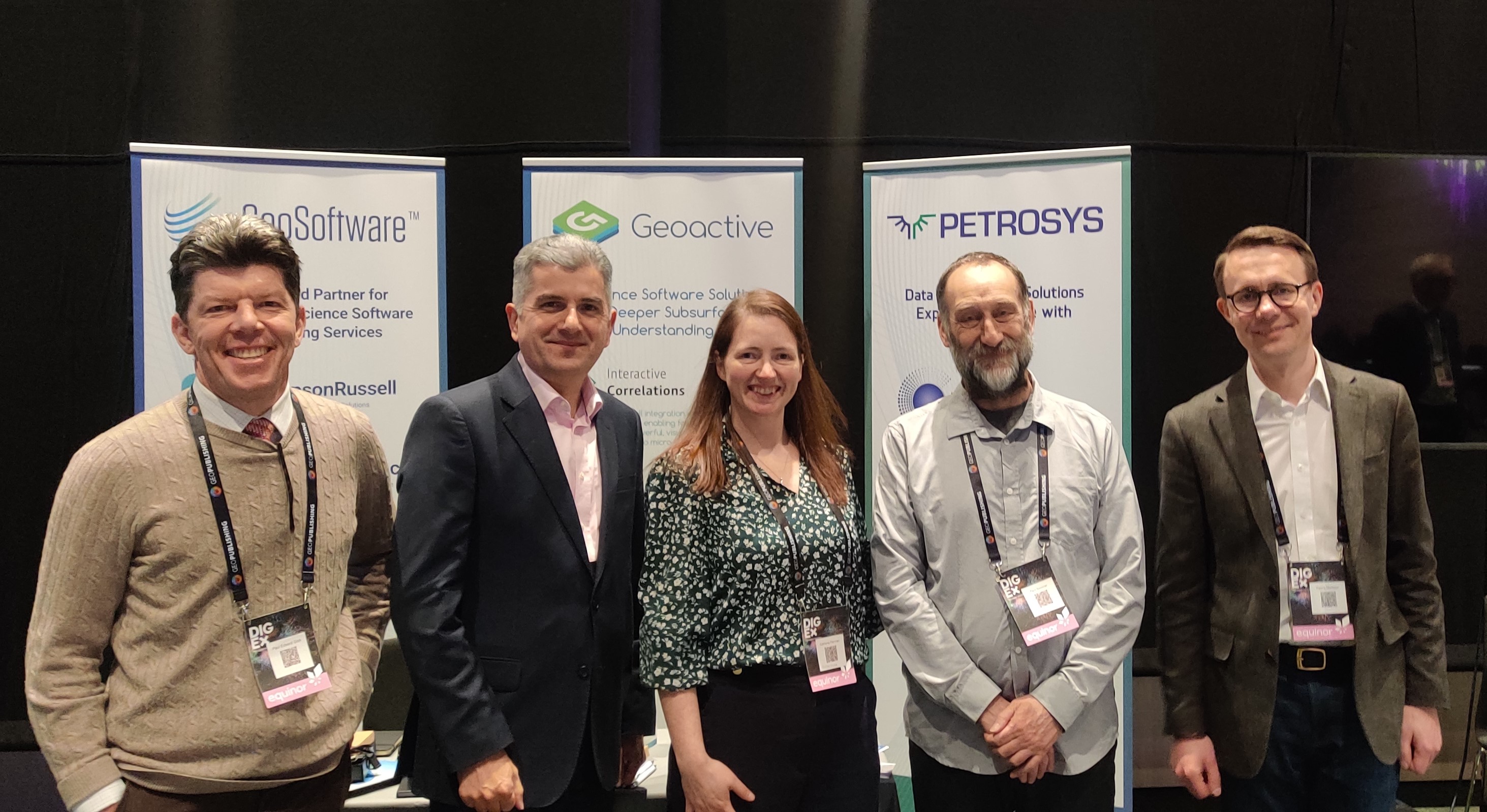
This project aimed to locate sweet spots on the Norwegian side of the Central Graben specifically for potential siliciclastic Paleocene hydrocarbon plays. Alenka Crne from Harbour Energy presented these findings at the DIGEX conference earlier this year and we want to thank her for her work with IC building upon the FMB data in achieving these observations.
Integration of data from multiple sources is a fundamental element that makes IC a fast and effective exploration tool. Utilising the mapping and visualisation of well data within IC has opened the doors for building more confident interpretations to achieve near field exploration goals.
Our website hosts a lot more detail of the different tools available within IC as standard as well as the more advanced stratigraphic and monitoring tools.
The acquisition and reprocessing of seismic data have grown over since exploration began in the North Sea to the point we cannot imagine exploration without utilising it extensively. As a result, it can be easy to overlook the subtle power of well data. By ignoring or downgrading the input from well data in preference of seismic, can result in expensive and ineffective modelling or completely overlooked potential within a play. Well data provide a ground truth that should serve as the foundation for play analysis.
The best way to revitalise old data requires integration of well data alongside seismic. Giving well data equal weight to seismic data leads to better understanding and higher confidence in your subsurface interpretation making any future steps or investment options more palatable.
The proven Siliciclastic Paleocene play is responsible for multiple oil fields across the Central Graben in the North Sea. For example, the Cod Field discovered in 1968 within turbidite deposits and the Forties Field, discovered in 1970 within stacked submarine fan sands. Initial development of the Forties field resulted in more drilled wells and additional data acquisition from the Paleocene. This provided a clearer understanding of the facies variations initially identified.1 Forties was initially expected to run dry by the early 1990’s but is now expected to run another 10 years2. This is an example of where more data from additional drilling can result in refined interpretations and build more confident understanding of the potential in an area.
Integration of log data, core data, pressure and production data can lead to practical and efficient correlation and mapping across a region. This would not be possible without continued investment in drilling and combining new data, new thinking and new technology with the previously collected data.
The demand for energy continues to grow, as does the demand for ‘clean energy’ and ‘sustainable energy’. All associated with the North Sea are building a deeper understanding of the plays that could contribute to the reduction of greenhouse gas emissions. Both continuing more efficient production of oil and gas and the discovery and evaluation of carbon storage require looking closer and with a new lens at the North Sea plays.
Completing exploration projects, from the regional play analysis to individual prospect studies, a structured and transparent database feeding a software application like IC is key. Being able to search for and visualise any data together at any scale can lead to updated interpretations to ensure consistent and effective understanding from well to well.
As part of a large, cross-border Play Analysis of the North Sea Central Graben, conducted by Harbour Energy, it was easy to pull more than 700 wells together to map and analyse the siliciclastic Paleocene Play.
Building a single database system in IC by importing data from FMB, national authorities datastores and files provided a powerful visualisation and interpretation platform. IC enabled the team to screen and work with well data at various scales which provided the freedom to add and evaluate not only data quality, but interpretation variations. This allowed a clear evaluation of each play, in this case, the Paleocene, in order to identify sweet spots across the area.
The Paleocene play evaluation incorporated assessing the Reservoir, Charge and Seal. Injecting new understandings and views on over 713 wells with lithology, core porosity and permeability, and depositional environment, enabled Harbour Energy to not only map out reservoir presence and quality, but the distribution and quality of the seal above as well. Integrating the hydrocarbon/fluid show information showed that almost one-third of these wells receive charge into the Paleocene stratigraphic zone.
Mapping the relationship between each well in the Central Graben showed a simplified lithology breakdown within the Paleocene zone found in each well alongside the hydrocarbon fluids/shows data. The variable height of the lithology columns shows the relative thickness of the Paleocene across the area based on True Vertical Depth (TVD). The hydrocarbon Shows are plotted in the bubbles at the well locations and show the proportion of the Paleocene with hydrocarbon present. It should be noted that the map only shows the wells that had lithology data from FMB.
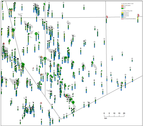
Figure 1: Central Graben map highlighting Palaeocene gross lithology variation downhole and the hydrocarbon type and relative presence within the Paleocene.
After spending the time and money drilling and collecting data from new wells, it is important to utilise it. Integrating data from multiple disciplines allows you to gain deeper understanding from measured data and can led to identifying previously overlooked plays. To achieve a clear understanding of your subsurface, the data should be pulled together and evaluated in tandem rather than in isolation. IC enabled Harbour Energy to do just that.
Pulling in data from multiple sources including NPD and FMB, Harbour were able to map the well locations and highlight the study area using the IC Map. Generating a simple well query identified 717 wells out of 778 host Paleocene intervals within the study area.
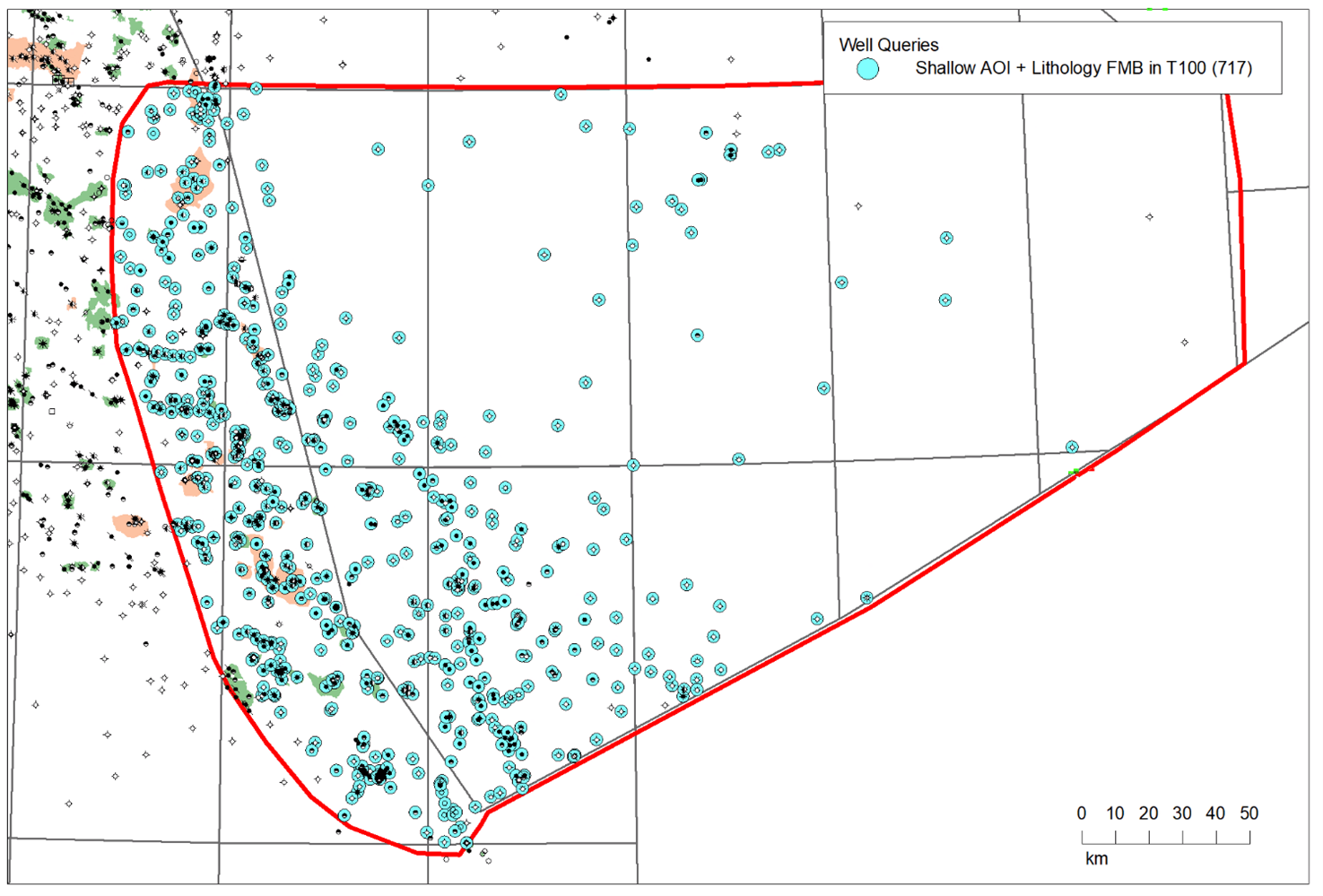
Figure 2: Paleocene presence from the NPD Diskos and FMB data sources.
Setting up Stratigraphic Schemes within IC sets the rules for the well data to validate against. It allows for fast and effective visualization downhole or on a map that highlights potential issues in each well.
Utilising the comparison of different interpretations of the stratigraphic zones can evoke questions or highlight nomenclature differences from well to well.
To establish the validity of data in an easily comparable way, new data were built to allow for simple queries to identify the same zone within each well, regardless of original naming or precision.
Any questions that arose can be addressed when examining the data vintage, source, confidence or comparing with other data to ensure the interpretation is valid. Where the wider data leads to modification, it can be done directly.
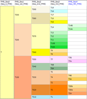
Figure 3: Stratigraphic Scheme built within IC using the standardised unit names and depiction colours as set by Harbour Energy.
Using the Stratigraphic Schemes, it was easy to build additional data to group the sequences into parent sequences to allow a larger scale review.
The original FMB lithology were simplified from 39 unique terms to 7 to differentiate the basic differences through the wells. This allowed for the review to be generated at different scales, regional review and wider correlation.
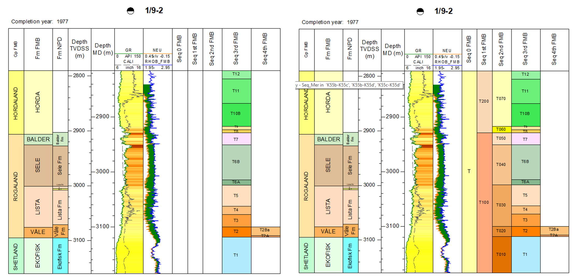
Figure 4: original data on the left from FMB and NPD for comparison and the generated zones based on the Stratigraphic Scheme rules applied to the well on the right. This allows for the entire T100 zone to be evaluated in one across the wider area.
The thickness of sandy lithologies within the T100 Paleocene zone was mapped from the 717 wells to show the variation and sandy lithology variations across the median line. Not surprisingly, the thickest Paleocene sands were seen in the UK side. Beyond reservoir quantity, the quality (porosity and permeability) plays a part in Play viability. Out of 717 wells, 106 had core porosity data and only 49 had permeability data as well.
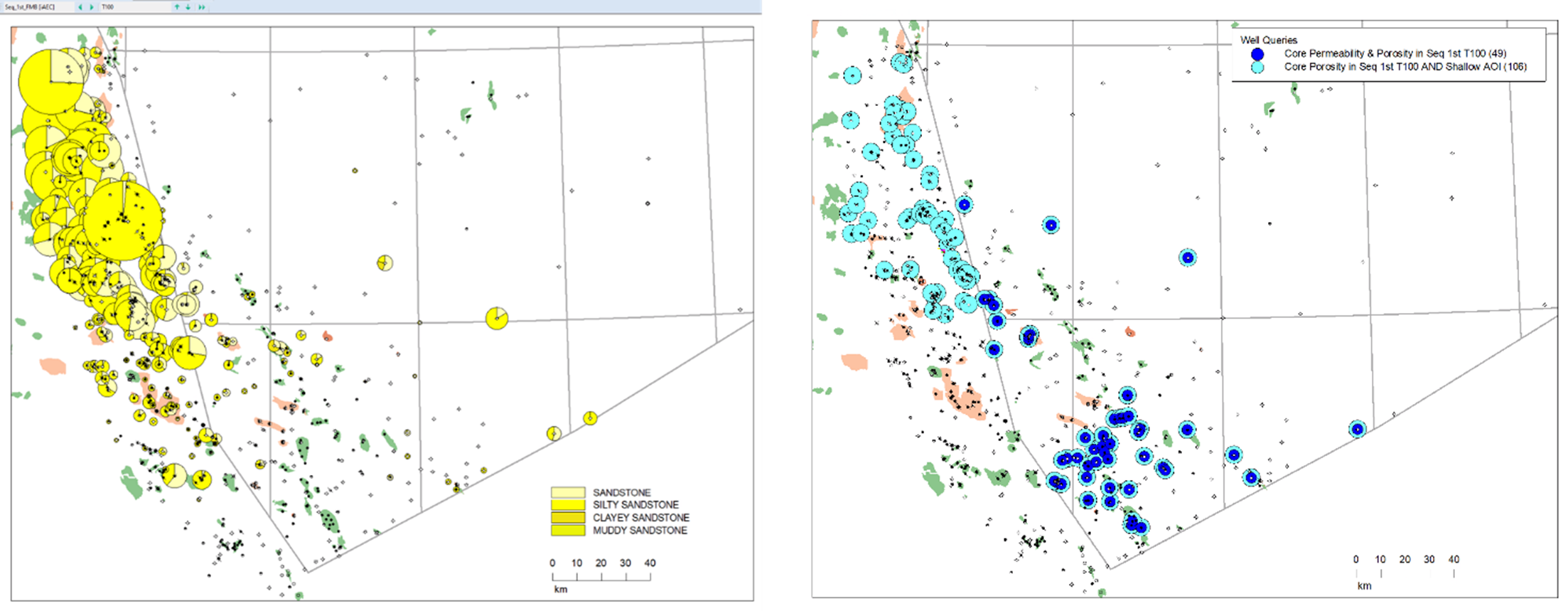
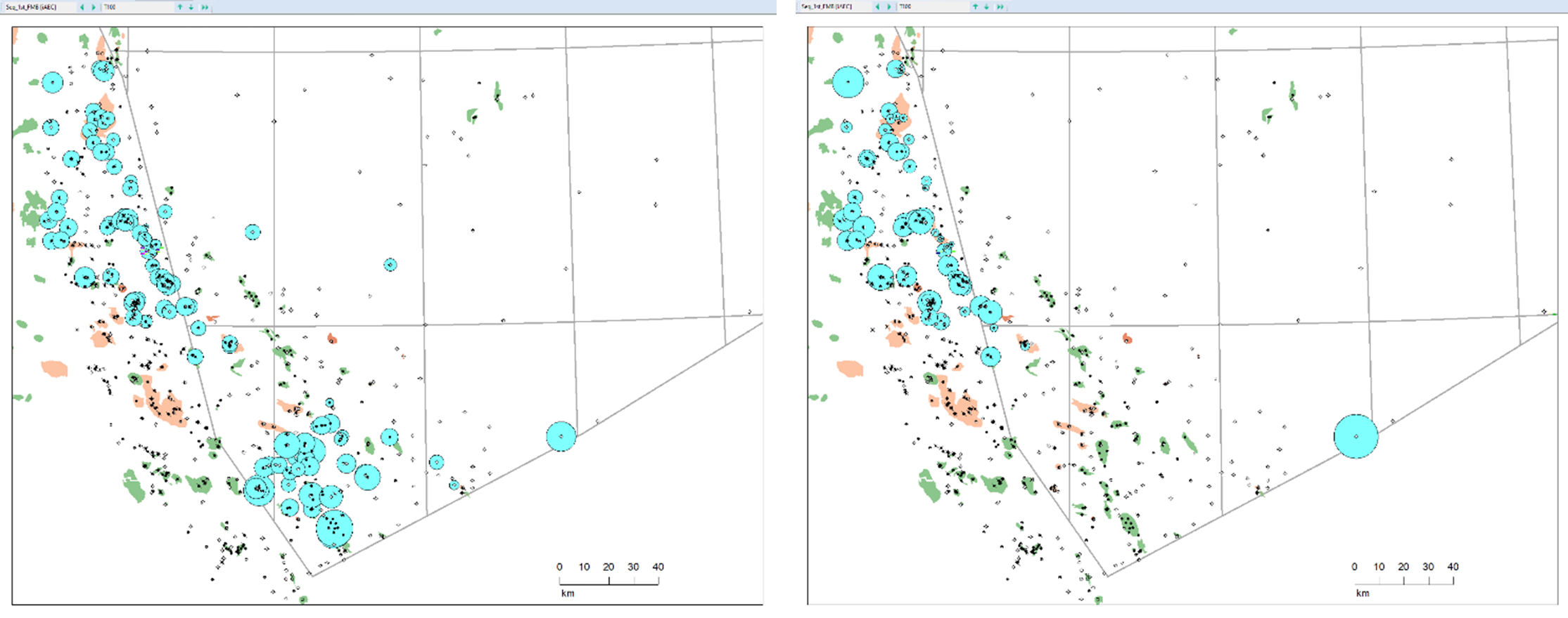
The average porosity of the Paleocene (T100) showed higher values on the Norwegian side. However, when focussing on the Paleocene sandstones only, the core porosity data drops from 106 to just 65 wells. Once again, most of these wells are in the UK sector, indicating the higher porosities in Norwegian wells are in Chalks.
One well stood out on the Norwegian side with a high porosity so a closer look was required. Well 3/6-1 showed the highest porosity by far within the Paleocene Sandstones on the Norway side of the Central Graben. Reviewing a range of data together can highlight if the data points rendered are anomalous or real. In this case multiple measurements were made ~35% for that cored section of the Palaeocene sandstone.
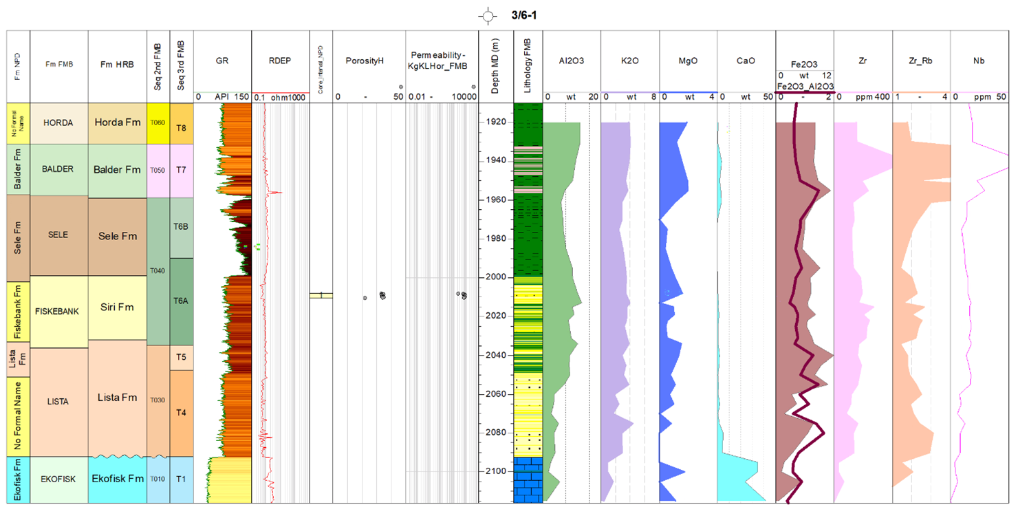
Figure 9: Digging deeper into the well data. comparing and displaying data coverage and determine the confidence level to hold in the anomalous measurements, like a high porosity within a Paleocene sandstone (lithology, porosity and permeability data from FMB; XRF data from the NOROG project Released Wells Initiative).
Digging deeper into the 49 wells with both porosity and permeability data, the lithological differences plotted on a scatter graph show a clear and not surprising different trends for sandstones and carbonates.
Directly Download this Case Study
However there were a number of data points showing high permeability mudstones which leads to the question, how do we explain that? Is there a mistaken lithological interpretation in these zones or have we some depth shift to apply that hasn’t been applied? Identifying the wells these points originate lead to answers.
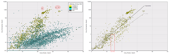
Figure 10: Porosity vs permeability plots. Lithological differences highlighted in colour and the Sandstone points highlighting a 15% vs 12.5% cutoff range at 1mD using the linear and exponential trendlines (porosity, permeability and lithology data from FMB).
Filtering out the noise and focusing on the sandstones within the Paleocene, using a cutoff of 1mD, the trends observed gave a minimum porosity of 12.5 and 15% (Figure 10 above). The 65 wells with porosity data were plotted to show the variation in depositional environment at depth. Using a porosity of >12.5% and depth above 3500mTVDSS as the favourable range, the data plot across all depositional environments. Wave-dominated shoreface environments appear to maintain higher porosity at depths closer to 4500m TVDSS above that 12.5% cutoff.
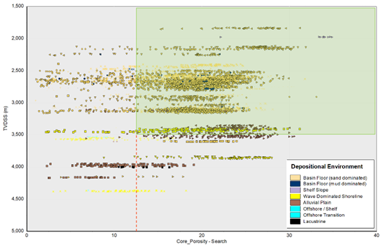
Figure 11: Porosity depth plot of all available wells highlighting the favourable porosity and depth in the green box, above 12.5% porosity and < 3500mTVDSS (porosity and depositional environment data from FMB).
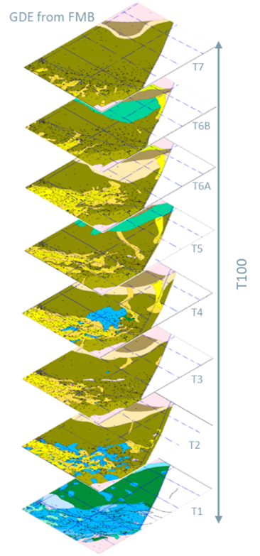
The Paleocene reservoir was mapped to show the Chance of Success (COS) using the Gross Depositional Environments (GDE) maps from FMB (miniature stacked images here), the lithological interpretation and the core data within the wider stratigraphic interpretation of the study wells.
This traffic light map shows the likelihood of encountering favourable Paleocene across the area where Green is likely, and Red is least likely.
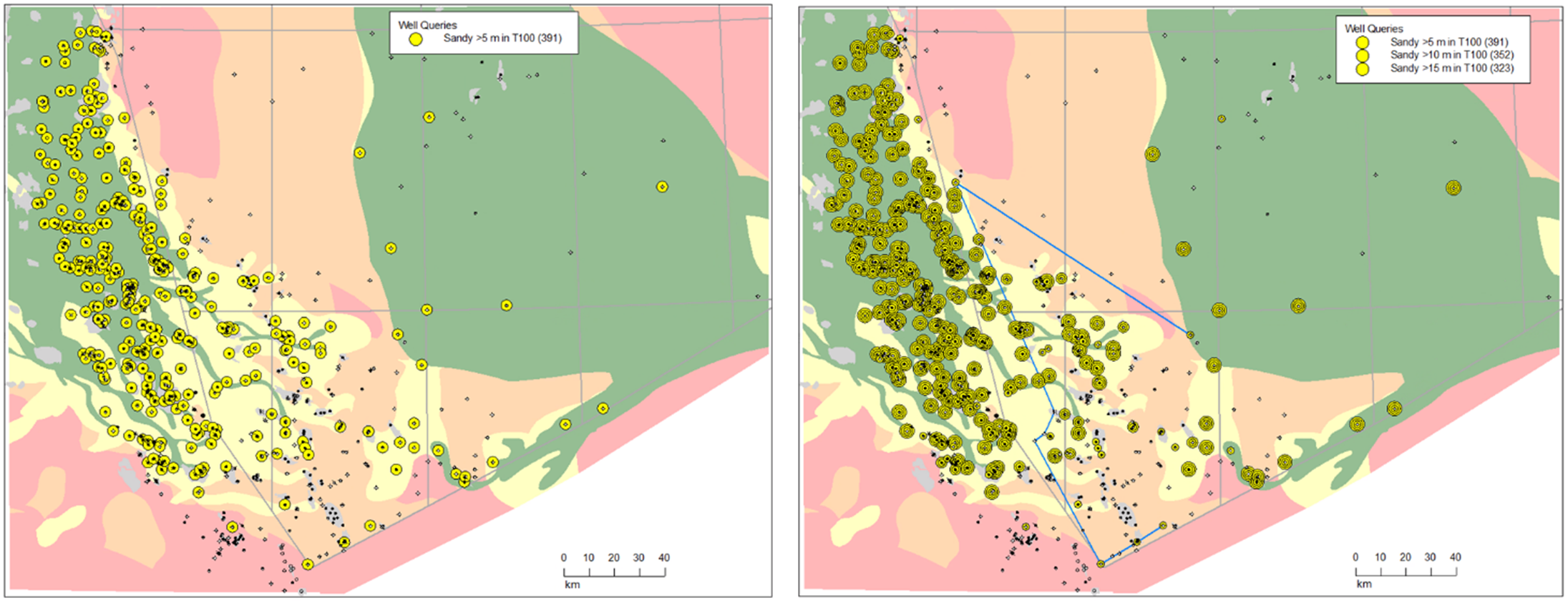
When we modify the thickness of cumulative sandstones cutoff within the T100 zone in each well, we see the number of wells drop from 391 with > 5m to 323 with >15m. The maps suggest an area on the Norwegian side might be worth looking at more closely.
Correlation is at the heart of IC and can provide the visualisation that leads to a deeper understanding of your subsurface. Looking at a representative section across the COS map can help QC the mapped areas for reservoir presence and thickness downhole. The yellow areas show lower likelihood of success than the green for the Siliciclastic Paleocene indicating sandstone is present, just perhaps not the desired quality or quantity. The orange areas show an even lower likelihood of finding a Paleocene reservoir indicating a lack of sandstone presence. However, looking at the wells in a correlation, it is possible the GDE maps need to be reassessed or the interpretations adjusted because we see sands with a greater cumulative thickness in some orange zoned wells while some yellow zones wells show no sand at all.
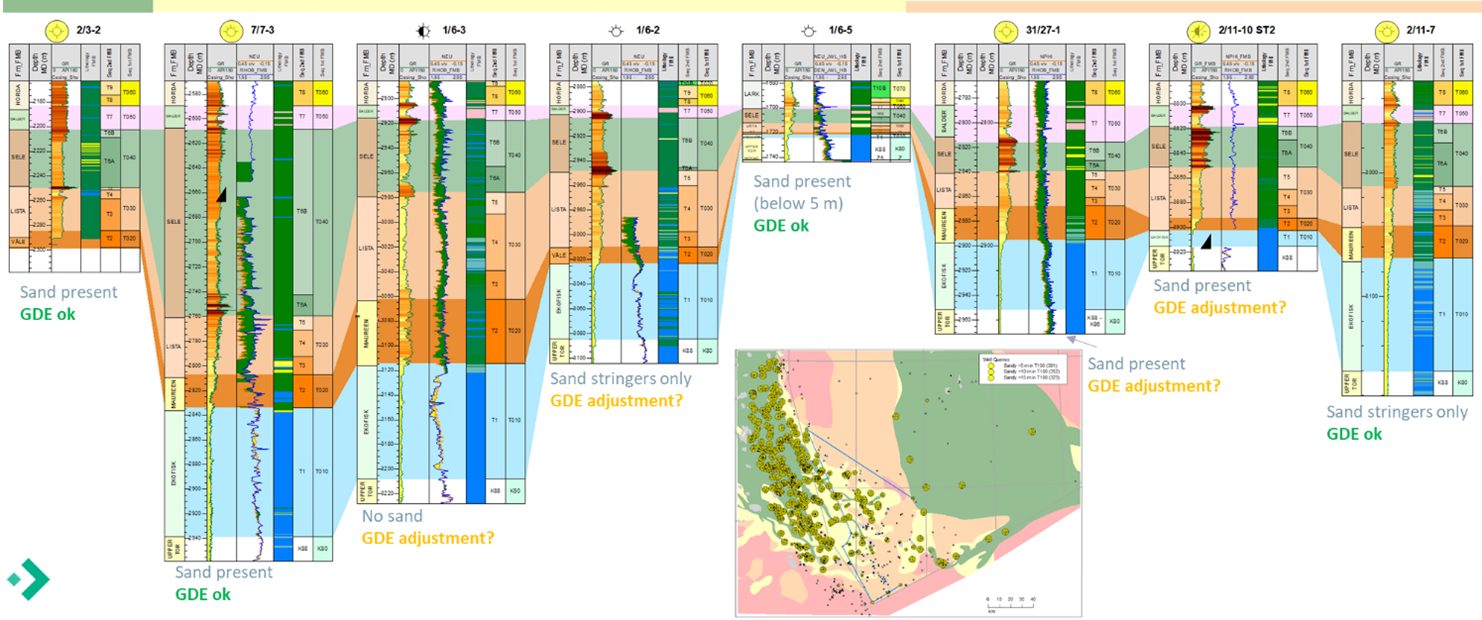
Figure 14: Correlation across the Norwegian wells highlighting questionable elements when comparing the Paleocene presence with the chance of success map.
Another key element on the petroleum system is the presence, thickness and quality of the seal. Equating mudstones to seal, it was easy to map the chance of success for each Paleocene Sequence using the sequence above’s mudstone percentages.
Gridding the inter-well prediction of mudstones and colouring with that same traffic light system as the reservoir, the likelihood of the seal presence and quality can be mapped easily within IC. When plotted alongside the specific well breakdown of the mudstones, showing the percentage of the sequence that is interpreted as mudstone with the size of the bubble representing the relative thicknesses, it is easy to identify where the seal play element poses a higher risk.
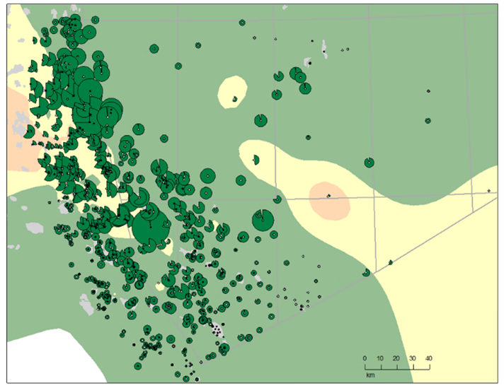
Figure 18: T30 (Lista) Reservoir sits below the T40 Sequence (lithology data from FMB).
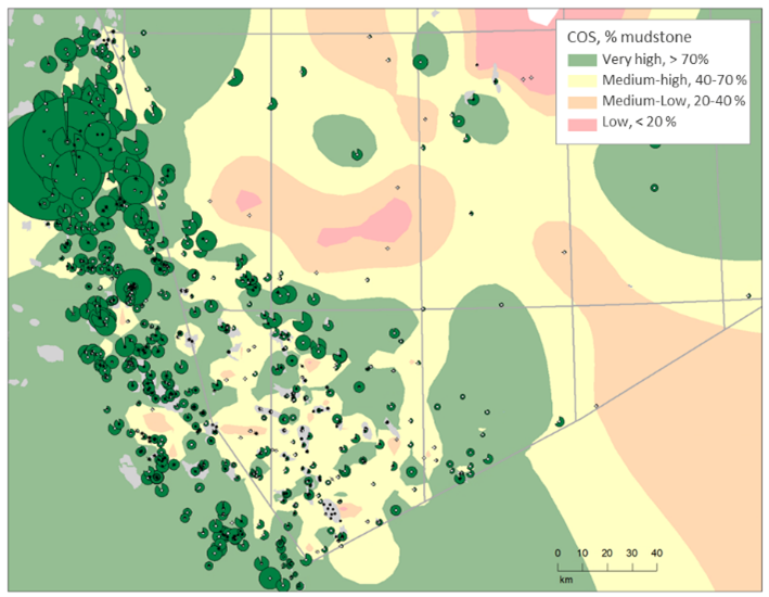
Figure 15 T40 (Sele) Reservoir sits below T50 Sequence (lithology data from FMB).
Mapping the hydrocarbon fluids/shows across the area resulted in a breakdown of oil, condensate and gas. Oil was found in 24% of the wells in the dataset. That’s 171 wells. The condensate was found in only 12 wells, which equates to ~1%, while Gas was found in 140 wells, that’s 20%. Since a number of wells contains both oil and gas, the percentage of wells containing any kind of shows is 33 %.
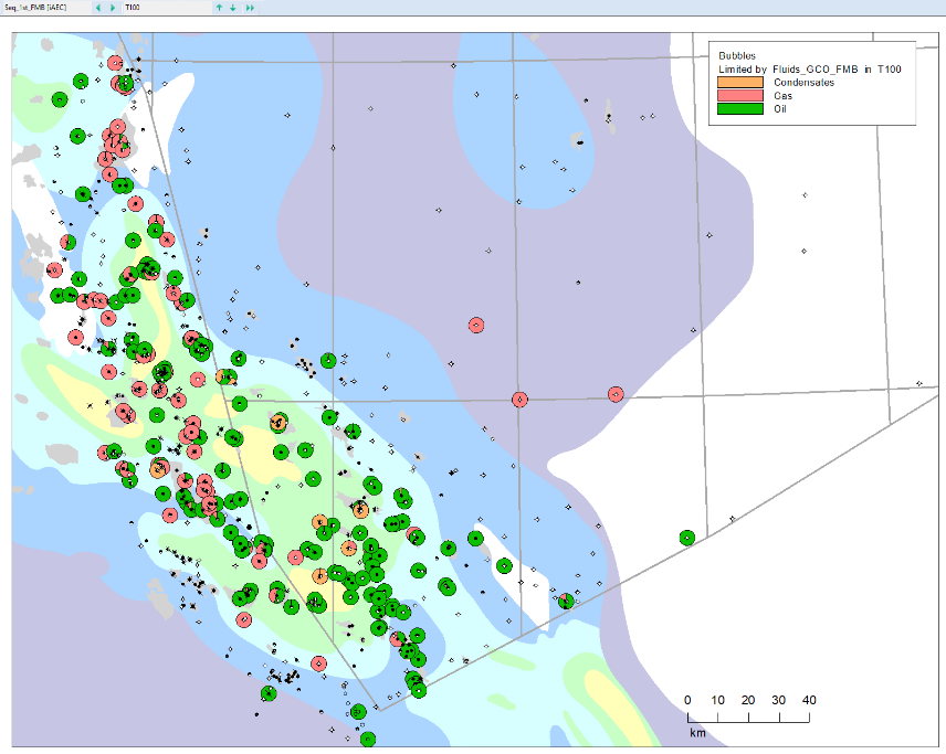
Figure 19: Mapped Kimm. Clay maturity using Vitrinite Reflectance (Millenium Atlas, 2002) alongside the presence of hydrocarbon fluids from FMB within the T100 Paleocene.
1 Carman, George & Young, Ray. (1981). Reservoir Geology of the Forties Oilfield.
2 Jane Whaley, (July 3, 2010). The First UK Giant Oil Field, GeoExpro
To determine the potential within the Siliciclastic Palaeocene Play across the Central Graben, the team at Harbour Energy used IC to integrate FMB data with proprietary and historical data from 351 Norwegian Wells and 427 UKCS Wells (and sidetracks).
Understanding, not only the seismic scale, but also the well logs, core, and cuttings scales of data can highlight previously overlooked areas. This example for the Paleocene play in the Norwegian Central Graben demonstrates that with the right tools, a properly structured database such as FMB and a software like IC that allows for analysis and visualisation at various scales, it is possible to quickly aid the decision whether a company should enter a play.
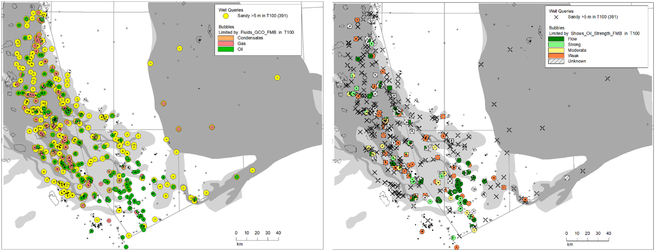
To identify the potential sweet spots for the Paleocene in the Norwegian Central Graben the data was filtered to show not only the presence of hydrocarbon in the Paleocene, but the relative strength of the shows as well. Utilizing the integration and visualisation tools available in our software, Harbour Energy were able to map and understand, not only the available data, but the impact alternative interpretations would have on the play prospectivity as well.
Interactive Correlations enabled that integration of multiple data to pull the spatial and zonal evaluations together and present them in a concise manner. Identifying where the well data did not match mapped interpretations shines a light on the potential for assumptions to influence the current understanding of a mature basin like the North Sea and highlights the vital need to continue to explore and evaluate each play in details in a similar way.
The latest version of Interactive Correlations (IC), our multi-well collaboration software, is now available. With two decades of continuous software...

Ask most people where North Sea decommissioning gets stuck and they’ll point to rigs, vessels, or the supply chain. They’re not entirely wrong – but...
This years DIGEX conference hosted by GeoPublishing was held in the winter wonderland of Oslo, Norway during the last week of March. It was an...