We spend somewhere between 50% and 90% of our time on a project getting the data ready and checking it (McDonald, 2021). Everything we build afterwards stands on that work, whether it is a petrophysical interpretation, a saturation height model or a facies model.
It is worth the time because errors do not stay still. A washed out density interval becomes a porosity error, the porosity error becomes a saturation error, and by the time it reaches a volume or a well placement decision nobody can see where it started.
What makes it difficult is that log data arrives looking like a completed and finished product. The curves are all there, the file loads, and a quick plot looks like a well should. Only when we go further into the data do we start to find out what state it is actually in!
The cost of a missed interval has gone up
If we look at plots of the data it can be easy for us to identify washed out sections, however, when we try to scale that workflow to 1,000 wells or even 10,000 we end up relying on an automated model to run that workflow. This can lead to intervals being averaged, skipped or mis-identified. This then feeds into an AI model to train on. If it is not spotted early on it is carried into every prediction the model makes afterwards.
None of this is unique to subsurface work, and the cost of it has been measured in other domains.
More than 25% of organisations report losing over $5M a year to poor data quality, 7% put their losses above $25M, and 43% of chief operations officers now name data quality as their top data priority (IBM Institute for Business Value, 2025). Unity lost $110M after bad data corrupted its machine learning models (Unity, 2022).
We have measured it on our own data as well as part of a wider study. We trained three models to predict a curve, then removed training data at random and watched the error climb. Random Forest barely moved across the whole range. Support Vector Regression drifted up steadily. The neural network held to about 60% missing and then degraded sharply (McDonald, 2021).
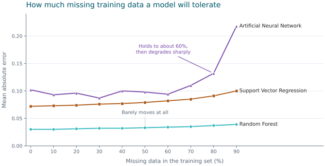
Figure 1. Error against missing data in the training set. How much it costs depends on the algorithm, which is worth knowing before choosing one for a sparse field.
Gather, align, flag, compare, repair
We can work through 5 different stages for our QC process:
Gather the curves, standardise the names and units, and find out what is missing. Although, it should be pointed out that standardising the names can lead to provenance of a curve being erased, as often the curve name can be a clue to the tool or process that created it.
Align the runs to ensure that data is depth with each other and with the reference curve, usually gamma ray.
Flag the intervals we can’t trust.
Compare the wells against each other instead of reading them one at a time.
Repair last. If we did this step early on, we may end up repairing the wrong data and using up valuable time.
Four of the above steps can leave us with a tidier dataset, however flagging is something that leaves us with a record of what is wrong with the data and how it may have been repaired.
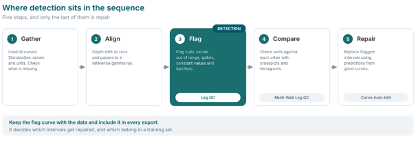
Figure 2. Repair comes last. Flagging comes third, where the record of what is wrong gets made.
What we flag
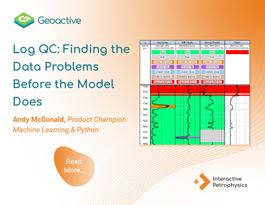
In IP's Log QC module we apply a set of rules to the data: identify nulls, highlight values outside a physical range, spikes, constant values where a tool has stopped responding, and intervals where the hole condition makes the reading unreliable.
At this stage we are not training a model, so nothing is learned. We are explicitly using our domain expertise to set the limits, and once set we can apply them on every well, so that we can easily view the plots for those wells to quickly visualise any errors.
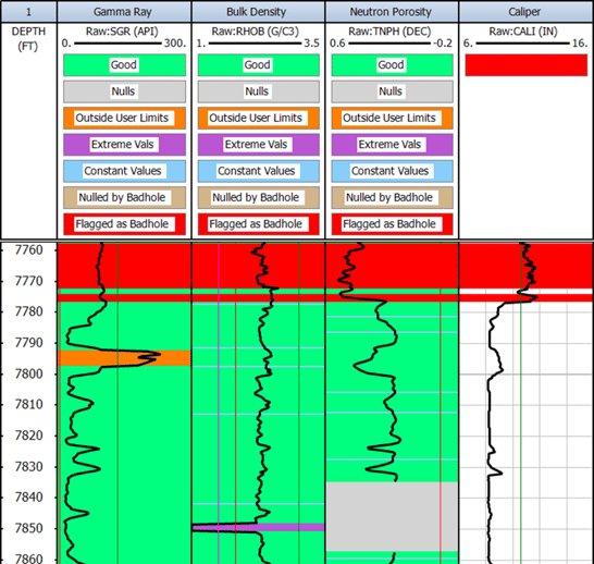
Keep the flag Curve with the data
Flags are the first thing in a dataset to get lost. One of us makes them, exports them, and the next person loads the data into a new project and the curves are dropped as the other person does not recognise them or decides they are not relevant to their work. Whilst this may result in a tidier dataset, it can lead to the loss of the reasoning behind the data issues that were identified or repaired.
One solution is to name the curves so they explain themselves and then keep them beside the curves they describe. That costs noting to very little at the time, and it also saves the next person repeating a day of work, or worse, not repeating it and going ahead with invalid data.
What the flags feed
A flag in IP is not a note to ourselves. It is an input that other tools read.
On a crossplot it helps discriminate the data, so points we already know are bad stop influencing what we see. In Curve Auto Edit it drives the repair: Auto Edit fits regressions from the curves that are still good and replaces only the intervals we flagged, leaving everything else as it was. For a machine learning model it filters the training data, which decides what the model gets to learn from.
That last one is where the cost sits. Every interval we flag as unusable is an interval that leaves the training set, and figure 1 shows what losing training data does to a model. Flagging finds the bad data. It also tells us how much good data we have left. That number decides whether a model is worth training at all.
Where to start
Flag before you repair, and flag before you train anything. Write the rules down as a rule set instead of carrying them in your head. Keep that rule set with the field rather than with the project. Export the flag curve with everything else.
None of this needs new software. It needs us to treat detection as work that produces something, rather than a look we take on the way to something else.
Three things to take away
- Detection is not repair, if you miss it or ignore it in a bad interval then it can reach a calculation.
- We write a rule set once and apply it to every well and adjust it where needed.
- The flag curve is the deliverable. It decides what we repair and what we train on and if it's left in the project we made it in, its meaning is lost.


 Andy McDonald


 Andy McDonald : June 12, 2025